Pivot Tables - a new Spin on your Data

Pivot Tables are a powerful tool for analysing your data

(Note: The method for building pivot tables is slightly different in Excel 2000 than it was in earlier versions of Excel.

Click here if you are using an older version of Excel)

Open the spreadsheet file WINELIST.XLS.

You are going to create a table showing how many wines we have by CATEGORY and YEAR.

Move the cell cursor to J1

Select the Data menu and choose PivotTable and PivotChart Reportoption.

The PivotTable Wizard will lead you through the task of setting up a Pivot Table.

In Step 1 click the Microsoft Excel List or Database and the Pivot Table options then click Next.

In Step 2 you specify the data that you want to summarise, including the row or column headings in the range.

5 In the Range field, type A1:H49 and click Next.

In Step 3 you specify where the pivot table will appear on your spreadsheet

Click Finish.

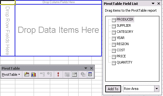
Your spreadsheet should now display the Layout and the Pivot Table dialog box shown below.

This layout forms the basis for your Pivot Table design.

To build the table we drag items from the Pivot Table dialog box to the layout area.

1. Drag the Year item from the Pivot Table dialog box to the layout area marked "Drop Column Fields Here"

2. Drag the Category item from the Pivot Table dialog box to the layout area marked "Drop Row Fields Here"

3. Drag the Quantity item from the Pivot Table dialog box to the layout area marked "Drop Data Items Here"

You have now described the structure of the table.

Your finished Pivot table should be similiar to the one below.

Experiment and build more pivot tables by using combinations of different row and column headings.

---