Pivot Tables - a new Spin on your Data

Pivot Tables are a powerful tool for analysing your data

1 Open the spreadsheet file WINELIST.XLS.

You are going to create a table showing how many wines we have by CATEGORY and YEAR.

2 Move the cell cursor to J1

3 From the Data menu choose PivotTable.

The PivotTable Wizard will lead you through the task of creating a Pivot table.

4 On the first screen choose the Microsoft Excel List or Database option, select Next.

On this screen you specify the data that you want to summarise, including the row or column headings in the range.

5 In the Range field, type A1:H49 Select Next.

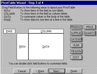
This window forms the basis for your Pivot Table design.

The column headings of the spreadsheet are displayed on the right side of the pivot table wizard window

.

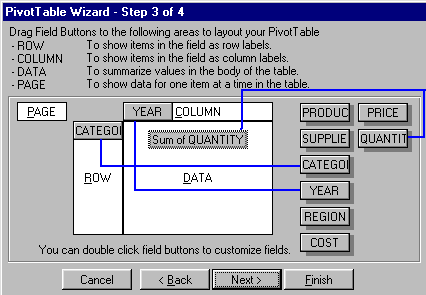
In this case you want the names of the YEARS at the top of the columns and the CATEGORY down the left side of the table.

In the data area you want the QUANTITY of bottles.

6 Drag the CATEGORY field to the Row area.

7 Drag the YEAR field to the Column area.

8 Drag the QUANTITY field to the Data area.

You have now described the structure of the table.

9 Choose Next.

Leave each of the options selected in this screen.

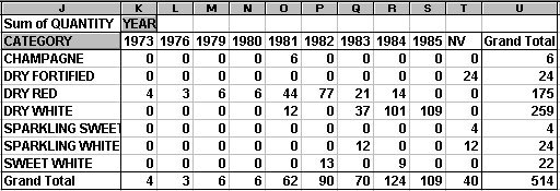
10 Choose Finish and you should now have a Pivot table similiar to the one below.

Build more pivot tables by using combinations of different row and column headings.

---